What
happens in the atmosphere during stadial-interstadial transitions?
H. Renssen, P.W. Bogaart & R.F.B Isarin
Faculty of Earth and Life Sciences, Vrije Universiteit Amsterdam,
The Netherlands
Introduction
In the North Atlantic region, the glacial climate was characterized
by rapid and abrupt climate swings between cold stadial conditions and
relatively warm interstadial conditions1-2 (often called Dansgaard-Oeschger
cycles). During these climatic shifts, the temperature increased by 9°C
within a few decades3-4. Stadial-interstadial transitions were
most probably caused by changes in the strength of the thermohaline circulation
in the North Atlantic Ocean5. Further study of these climatic
shifts and their impact on the envrionment is important, as this provides
information on the response of the geo-system during phases of rapid climate
change. We have used an atmospheric general circulation model (AGCM) to
study the change in atmospheric circulation during the last stadial-interstadial
transition: the shift from the Late Pleniglacial to the Bølling
at 14,700 yrs BP.
Model and experiments
The applied AGCM is the ECHAM4-T42 model6 of the Max Planck
Institute for Meteorology in Hamburg, Germany. For this study, we conducted
three experiments:
-
CONTROL: a control simulation of the present-day climate
-
BØLLING: a simulation with boundary conditions for the Bølling
period
-
LATE-PLENI: a simulation with boundary conditions for the Late Pleniglacial
The boundary conditions that were changed compared to CONTROL include
surface ocean conditions (SSTs and sea ice), orbital parameters, atmospheric
concentrations of trace gases, surface albedo, ice sheet extension and
topography. In the figure below, the prescribed anomalies in boundary conditions
for LATE-PLENI and BØLLING are shown.
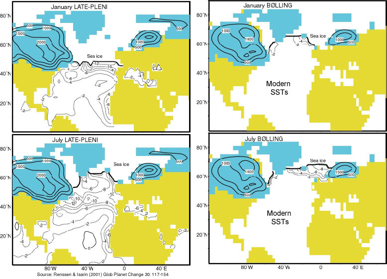
Boundary conditions in the North Atlantic region prescribed in experiments
LATE-PLENI and BØLLING. Yellow denotes land-surfaces, blue land-ice
and white ocean. The SSTs and ice-sheet elevations are plotted as anomalies
compared to experiment CONTROL.
Surface temperature
The simulated surface air temperatures clearly reflect the influence
of the prescribed changes in SSTs and sea ice cover. For instance, January
temperatures increase by more than 40°C over the central North Atlantic,
where a sea-ice cover is no longer present in the Bølling during
winter. Over the adjacent continents, the warming is somewhat less, but
still considerable.
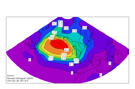
Simulated increase in January surface air temperature (°C) over
the 14,700 yr BP stadial-interstadial transition (BØLLING minus
LATE PLENI)
The simulated temperature increase for NW Europe (15 to 25°C), is
in agreement with reconstructions based on a variety of proxy data (see
Renssen & Isarin, 2001), indicating that the set of boundary conditions
prescribed in LATE-PLENI and BØLLING are based on reasonable assumptions.
This suggests that we may use these experiments to study the changes in
atmospheric circulation over a stadial-interstadial transition.
Sea level pressure
In experiment LATE-PLENI, the winter mean surface pressure over the
ice-covered North Atlantic Ocean is relatively low due to the strong surface
cooling and descending airflow. As a consequence, the Icelandic Low is
not well developed. In BØLLING, on the other hand, the surface pressure
distribution is similar to today with a strong Icelandic Low and a steep
pressure gradient over the North Atlantic. Over NW Europe, however, the
pressure gradient is steeper in LATE-PLENI than in BØLLING due to
the more easterly position of the Icelandic Low under stadial conditions,
producing stronger winds over the continent between 50 and 55°N in
LATE-PLENI. Thus, over the ocean, the westerly winds become stronger during
the stadial-interstadial transition, while over NW Europe the winds become
weaker. The latter result is consistent with geological evidence7,
showing a strong decrease in eolian deposition during last stadial-interstadial
transitions.
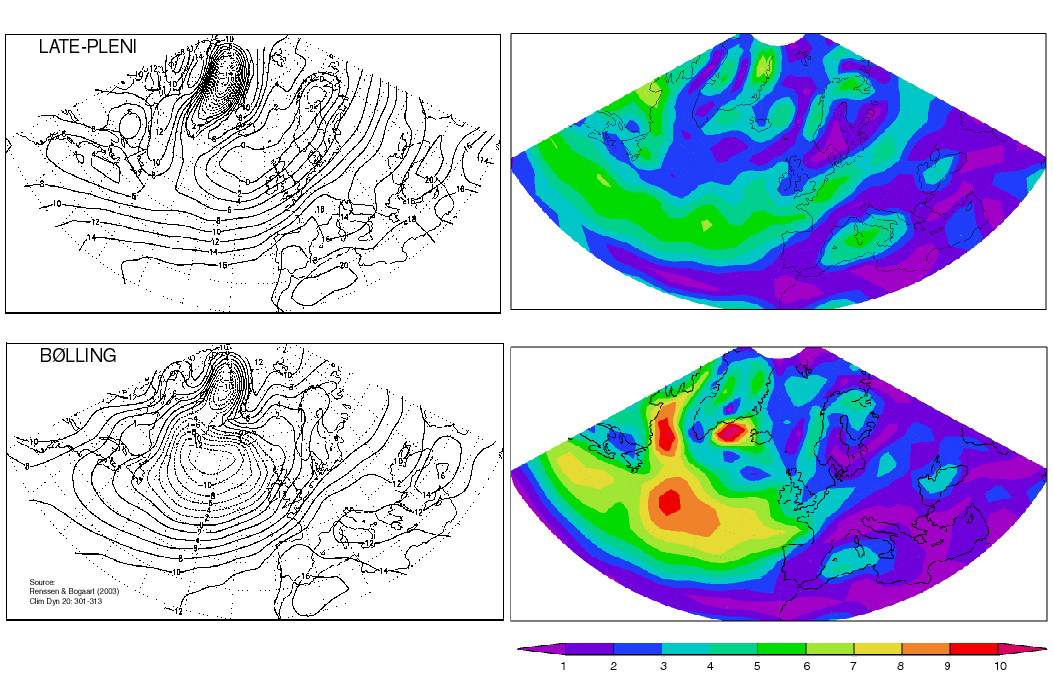
These figures show the simulated winter sea level pressures (left
panel) and wind speed (right panel, see scale bar in m/s). The surface
pressures are shown as anomalies from the global mean to account for pressure
differences related to the introduction of ice sheets.
Storm tracks
To analyze the changes in storm tracks, we high-pass filtered the standard
deviations of the sea level pressure. In LATE-PLENI, the storm track was
positioned along 55°N, following the main temperature gradient associated
with the southern sea-ice margin. A clear west-east orientation is visible,
indicating that depressions reached NW Europe very frequently. In contrast,
the reduced sea-ice cover prescribed in BØLLING produced a main
storm track with a southwest-northeast orientation, with depressions mainly
travelling into the Nordic Seas area. Thus, our experiments suggest that
NW Europe experienced a drastic decrease in storm activity during stadial-interstadial
transitions.

Simulated storm tracks for experiments LATE-PLENI and BØLLING
Effect on temperature variability
The noted change in storm activity had a major influence on the temperature
variability in NW Europe. In LATE-PLENI, the passage of a cyclone first
brought relatively mild Atlantic air to the European continent with southwesterly
winds, resulting in temperatures of 5°C. Subsequently, after the passage
of the depression, northerly winds transported extremely cold air to NW
Europe that originated from the sea-ice covered North Atlantic, producing
temperatures around 40°C. Thus, within days, the temperature in NW
Europe fluctuated between 40°C and 5°C. In BØLLING, the
temperature fluctuations were much smaller, although during cold outbreaks
the temperatures still reached 20°C and the mean winter value was
around 7°C. A further important difference with LATE-PLENI is that
during winter the temperatures regularly reached 3°C in BØLLING,
thus causing frequent melting of the snow pack, whereas in LATE-PLENI the
snow pack was able to build up throughout the winter.

Daily temperatures for one year, averaged over NW Europe. Note
the strong variations in LATE-PLENI, which are associated with the passage
of cyclones.
This difference caused substantial changes of the hydrology during stadial-interstadial
transitions, as in LATE-PLENI the runoff peaked in spring during the melt
of the thick snow pack, whereas in BØLLING the runoff was more evenly
distributed over winter. This change in runoff is consistent with geological
evidence suggesting that rivers in NW Europe changed from braided to meandering
systems during stadial-interstadial transitions8. Consequently,
our results suggest that the day-to-day temperature variability was strongly
reduced in NW Europe during stadial-interstadial transitions, which had
a strong impact on the surface hydrology here.
For further information, please consult the following papers
Renssen, H. & Isarin, R.F.B. (2001) The two major warming phases
of the last deglaciation at ~14.7 and ~11.5 kyr cal BP in Europe: climate
reconstructions and AGCM experiments. Global and Planetary Change30:
117-154.
Renssen, H. & Bogaart, P.W. (2003) Atmospheric variability over
the ~14.7 kyr BP stadial-interstadial transition in the North Atlantic
region as simulated by an AGCM. Climate Dynamics 20: 301-313.
References
-
Johnsen, S. J., Clausen, H. B., Dansgaard, W., Fuhrer, K., Gundestrup,
N., Hammer, C. U., Iversen, P., Jouzel, J., Stauffer, B., and Steffensen,
J. P. (1992). Irregular glacial interstadials recorded in a new Greenland
ice core. Nature 359, 311-313.
-
Bond, G., Broecker, W., Johnsen, S., McManus, J., Labeyrie, L., Jouzel,
J., and Bonani, G. (1993). Correlations between climate records from North
Atlantic sediments and Greenland ice. Nature 365, 143-147.
-
Koç, N., and Jansen, E. (1994). Response of the high-latitude Northern
Hemisphere to orbital climate forcing: evidence from the Nordic Seas. Geology
22,
523-526.
-
Severinghaus, J. P., and Brook, E. J. (1999). Abrupt climate change at
the end of the last glacial period inferred from trapped air in polar ice.
Science
286,
930-934.
-
Ganopolski, A., and Rahmstorf, S. (2001). Rapid changes of glacial climate
simulated in a coupled climate model. Nature 409, 153-158.
-
Roeckner, E., Arpe, K., Bengtsson, L., Christoph, M., Claussen, M., Dümenil,
L., Esch, M., Giorgetta, M., Schlese, U., and Schulzweida, U. (1996). The
atmospheric general circulation model ECHAM-4: model description and simulation
of present-day climate. Max-Planck-Institute für Meteorologie report
no. 218, Hamburg, Germany, 90 pp..
-
Kasse, C. (1997). Cold-climate aeolian sand-sheet formation in north-western
Europe (c. 14-12.4 ka); a response to permafrost degradation and increased
aridity. Permafrost and Periglacial Processes 8, 295-311.
-
Huisink, M. (1997). Late-glacial sedimentological and morphological changes
in a lowland river in response to climatic change: the Maas, southern Netherlands.
Journal
of Quaternary Science 12, 209-223.
BACK TO HOME
to publication list Hans Renssen
go to modelling of the 8,200 yr BP Holocene
cooling event
go to study on the termination of the African
Humid Period at ~6 kyr BP
go to simulation of the impact of global deforestation